Identifying Meaningful Change in Athlete Monitoring Data

Not All Normative Data Answer the Same Question

Athlete monitoring is often discussed in terms of whether an athlete is “within the (or their) norm.” But normal can mean several different things. It can describe how an athlete compares with other athletes of a similar group (age, gender, position), how an athlete compares with their own history, or how an observation compares with what is typical for that athlete under a particular set of circumstances.

Those are different questions, and they require different reference points. Therefore, it is vital that we are using the most appropriate reference point for comparison based on the question we are trying to answer. Furthermore, the analytical approach we utilize to compare athlete data to that reference point, and subsequently identify change, must be determined based on the question we are trying to answer while utilizing the most appropriate reference point to do so.

In other words, the value of normative data is determined by the question it is being used to answer.

For example, a countermovement jump (CMJ) can be used as an assessment of current performance and certain physical attributes following a training block, as part of an athlete profile to benchmark performance in comparison to a position group, or as a monitoring measure represented neuromuscular status and comparing the athlete’s performance with their own historical or context-matched data. Thus, the measurement does not determine the reference point, the question does.

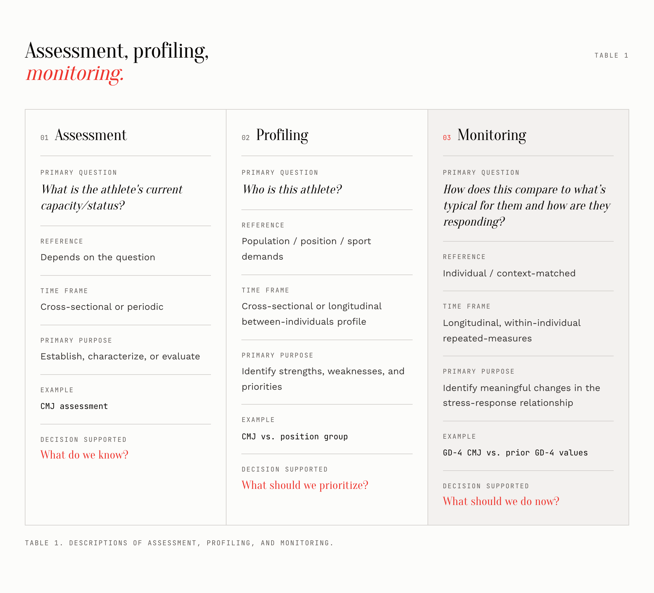
Assessment, profiling, and monitoring describe how we use the data, while the question we are trying to answer determines the normative data that we are comparing those measures against. Therefore, the same measure can serve different purposes depending on the question, timing, and intended use.

Monitoring is anchored in understanding the stress-response relationship (check out this post) and asks how the is changing or responding over time. Repeated, within-individual longitudinal data allows for the athlete’s own historical data to become the reference point, while using context-matched longitudinal data when appropriate. In the context of athlete monitoring, a couple of most significant benefits of having a strong within-individual longitudinal dataset is being able to more confidently identify change and patterns or trends in the stress-response relationship over time (Rebelo et al. 2026; Robertson et al., 2017; Ward et al., 2018).

Meanwhile, profiling asks who the athlete is relative to their peers within a given population such as within a sport, position group, age, or gender. Moreover, it asks what the physical demands and key attributes are for the athlete given their sport, position group, or job description. Population, positional, or sport-specific normative data can be used for describing characteristics, identifying strengths and weaknesses, and prioritizing training goals.    

Finally, assessments ask about the athlete’s current capacity or status. It is often point-in-time or periodic data and can be used to establish a baseline, characterize performance, evaluate an intervention, screen for deficiencies, or answer a specific performance question.

Not all data collection serves the same purpose. Assessment, profiling, and monitoring are complementary, but distinct. They all answer different questions, require different analytical approaches, and have different purposes. Confusing them can lead us to apply the wrong reference, or use a measurement collected for one purpose to answer a question it was never designed to answer.

Types of Normative Data Reference Points

I think about normative data reference points in three broad categories. The categories are defined by the question being asked, rather than by the statistical method used to calculate them.

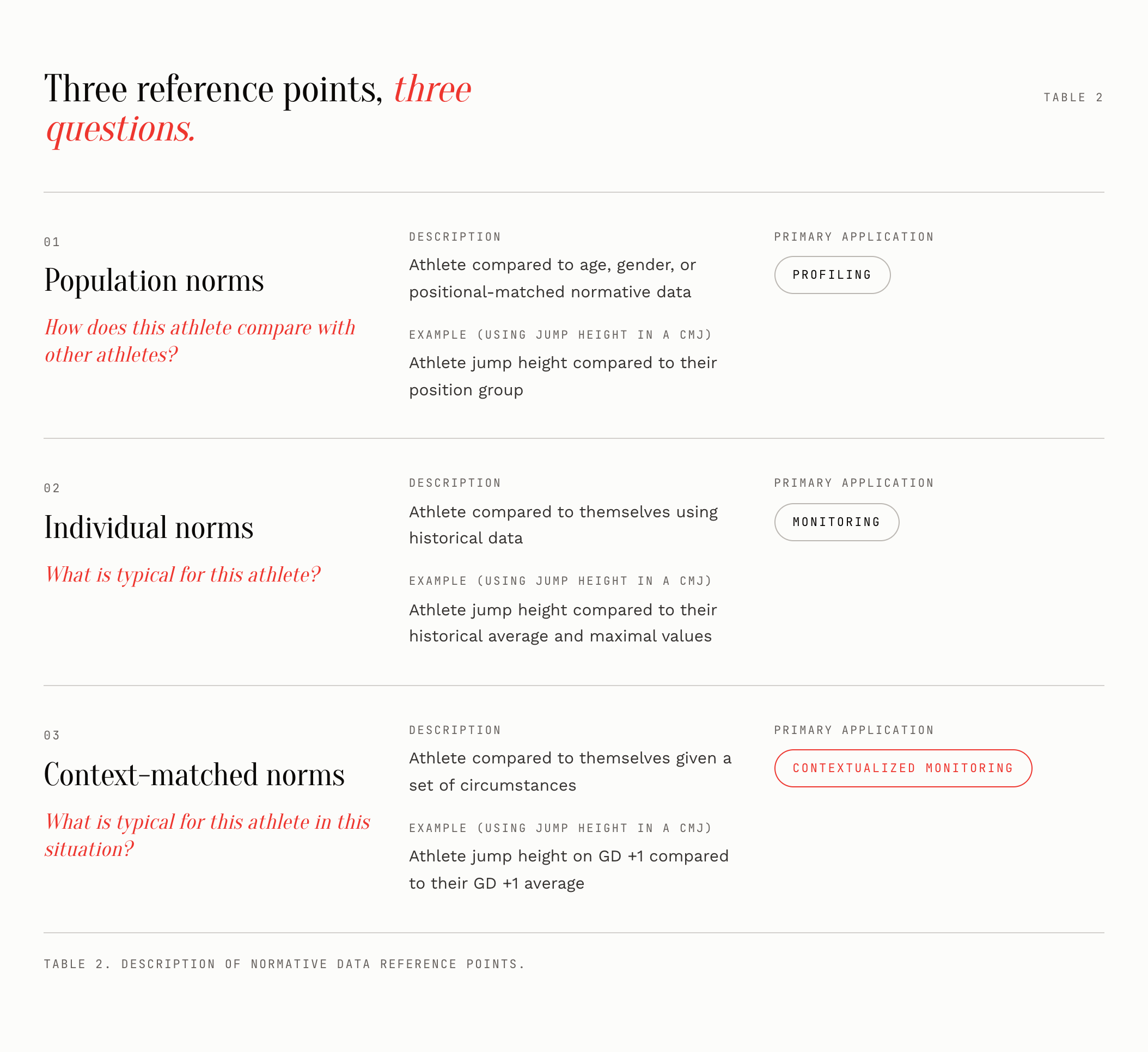
Population Norms – Primary Application: Profiling

Population or between-athlete norms answer comparative questions such as: where does this athlete sit relative to a given population? These data can be useful when comparing an athlete physical abilities or capacities to their age, gender, or position-matched counterparts. Moreover, these data can be useful when describing positional demands, establishing training goals, or understanding characteristics of a team or competitive population.

For example, an athlete’s sprint speed or reactive strength can be compared with other athletes at the same position, or a youth athlete’s relative strength can be compared to those of the same age and gender. Meanwhile, the game demands of a particular position group or job description can be used as a reference point to individualize a training program based on the expected game demands.  

However, a population average is not the appropriate reference for day-to-day monitoring at the individual level. If the question is whether today’s sprinting volume or CMJ performance is unusual for the individual athlete, comparing those values with a population group does not provide an appropriate answer.

Individual Norms – Primary Application: Monitoring

For monitoring, an athlete’s own longitudinal data is more informative than a population average. The athlete becomes their own reference point. This does not mean population or positional data are unimportant, but they simply answer a different question. Population data can help describe demands, establish profiles, and understand where an athlete sits relative to peers. Longitudinal individual data are more useful when the question is how the athlete is responding to the stress they are experiencing, or when attempting to identify patterns or trends over time (Robertson et al, 2017; Ward et al., 2018).

This approach applies to response indicators such as neuromuscular status, autonomic function, or wellness, but it also applies to the stress being imposed on the athlete. If we want to know whether a training stimulus is different from what an athlete is accustomed to, the athlete’s own training history provides an important reference.

Context-Matched Norms – Primary Application: Contextualized Monitoring

An individual norm becomes more useful when the reference is matched to the circumstances in which the observation occurred. A football player’s GD-4 workload is not necessarily comparable to their GD-1 workload. A regular practice week is not necessarily comparable to a short week. A training session during a congested schedule may have a different meaning than the same training session during a normal microcycle. That means the reference point itself should contain relevant context and be situated in similar set of conditions. This makes the data more relevant, while allowing practitioners to better identify changes in monitoring variables.

In my athlete monitoring framework, daily training stress comparisons are matched to relevant time points such as GD-4, GD-3, and weekly comparisons matched by game weeks or mesocycles (phases within the annual plan). Meanwhile, the reference point is rolling allowing for contextual changes rather than automatically fixed. If a player starts the year buried on the depth chart and playing only special teams but then transitions into a starting role with minimal special teams play, it would be inappropriate to compare his early season GD-4 high-speed running volume to his mid-season GD-4 high-speed running volume. Similarly, it’s inappropriate to compare a GD-4 workload that occurs during an unusual short week to a GD-4 workload on a normal week.

However, unusual observations should not automatically be deleted. They may represent exactly the context that needs to be understood. The practitioner should determine whether the observation represents a comparable training circumstance before allowing it to influence the reference data.

Understanding Variability

Once we choose an appropriate normative reference, the next question is: how much does that measure normally vary?

This is where variability becomes important. A mean tells us where the center of a distribution sits. It does not tell us how tightly the observations cluster around that center. Two athletes can have the same mean, while having very different amounts of normal variation.

Consider an athlete with 20 CMJ observations. Their mean jump height is 41.0 cm, and their standard deviation is 2.0 cm. Several different descriptions can be made from those data and each answers a different question.

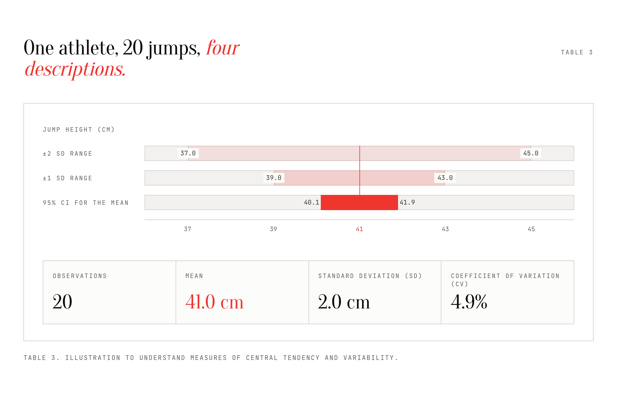
The mean of 41.0 cm is the athlete’s central tendency. The standard deviation (SD) of 2.0 cm describes the spread of the observations around that mean and the coefficient of variation (CV) expresses that variability relative to the mean. In this example, CV = (2.0 ÷ 41.0 × 100 = 4.9%).

Meanwhile, the 95% confidence interval (CI) describes the uncertainty around the estimated population mean. Often misunderstood, it does not describe the range in which 95% of future individual observations should fall. With 20 observations, the 95% CI for the mean is approximately 40.1–41.9 cm. A 95% CI around a within-individual mean becomes narrower as sample size increases with more repeated measures creating more precise intervals. However, this does not mean the athlete suddenly becomes less variable. It is simply describing the uncertainty around a specific individual’s (within-individual) true underlying mean (Bernards et al. 2017).    

Finally, the ±1 SD and ±2 SD ranges provide approximate descriptions of the observed distribution if the distribution is reasonably well behaved. They are not individual clinical or performance reference limits, and they should not be interpreted as universal decision thresholds. These ranges are helpful when identifying trends or patterns in monitoring data utilizing statistical process control techniques. The “two standard deviation band method” is used to set upper and lower control limits and allow a practitioner to quickly identify if an athlete’s data is deemed “out of statistical control” and warrants further investigation (Ward et al. 2018).

The important distinction is the confidence interval tells us about the precision of the estimated mean, while the standard deviation tells us about variability around the mean.

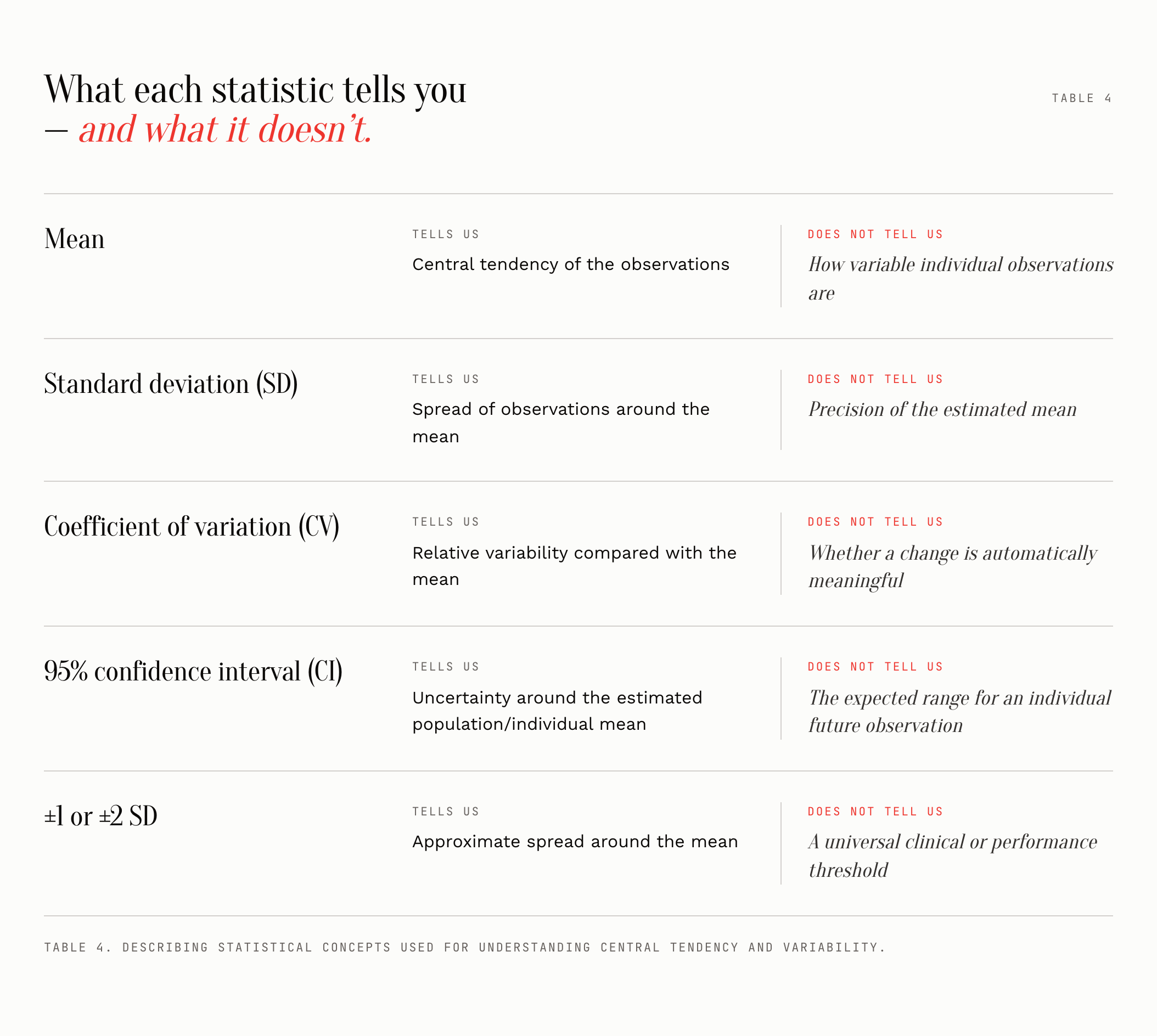
For monitoring, this distinction matters because our primary question is usually about the individual observation. For example, is today’s value unusual relative to what we would expect for this athlete? The confidence interval can help describe how precisely we know the athlete’s mean, but it is not the tool that answers that question.

Understanding Percent Change Relative Variability

Consider two athletes who both have an average CMJ jump height of 41.0 cm. If one athlete typically varies by 2.0 cm and the other by only 0.8 cm, a current value of 38.0 cm represents a very different deviation.

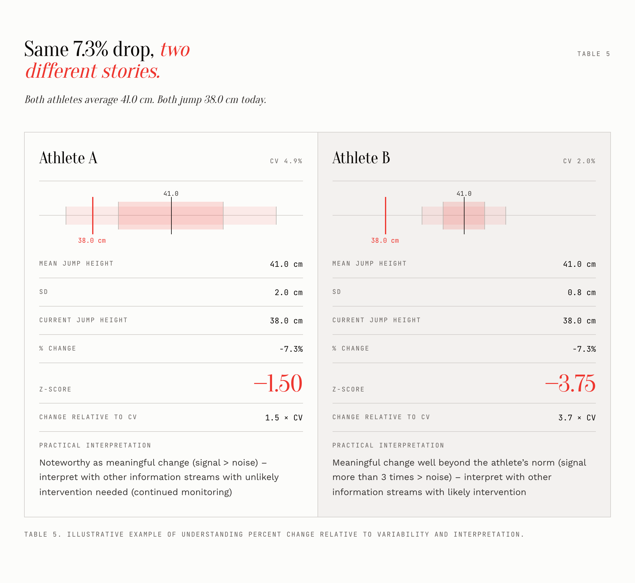
The observed change is identical with both athletes demonstrating a decrease of 7.3% in jump height. However, the interpretation differs between each athlete. Athlete A is 1.5 standard deviations below their mean, while Athlete B is 3.75 standard deviations below theirs. A percentage change tells us what changed, while variability tells us whether that change is unusual.

Normative Data and Analytical Approaches

It is useful to distinguish the normative reference data from the statistical description of that reference. The type of normative data selected is dependent upon the question we are trying to answer. Once we determine the most appropriate type of normative data to use, we then must determine the most appropriate analytical approach to utilize. The type of normative data indicates what we are comparing against, while the analytical approach determines how we are statistically making that comparison.

The standard deviation can quantify the spread around an individual mean or a context-matched distribution, while the coefficient of variation can describe relative variability. A z-score is useful way to determine how far from the mean a value is by number of standard deviations. Z-scores can be calculated comparing values from population means or individual means, and convert raw scores into a standard score. Meanwhile, the standard error of the mean (SEM) or the minimal detectable change (MDC) may be useful when the question concerns measurement error or the smallest change that can be distinguished from expected measurement noise (Bernards et al., 2017; Harry et al., 2024; Hopkins 2004). The latter are statistical methods used often for interpreting a reference, as opposed to comparing athletes to normative data. Therefore, the statistical method utilized should follow the question, as each of these methods describe a different aspect of the data and can be employed to create better analysis of the data.

Identifying Changes in Training Load Variables – Theoretical Framework

Similarly to the data already discussed, training load variables should also be interpreted relative to what an athlete has historically experienced.

The question is not simply, “How much did the athlete do?” It is also, “Is the stress we imposed different from what this athlete is accustomed to, and how might that influence the subsequent response?”

Training stress is the stimulus that disrupts homeostasis. The response to that stimulus includes some magnitude of acute and residual fatigue, as well as some type of decrement in the athlete’s current performance level until there has been a sufficient recovery window. When appropriately dosed and repeated over time, this process facilitates adaptation and supercompensation of the athlete’s level of performance. Classic theoretical models from Hans Selye and Carl Banister provide useful theoretical frameworks for thinking about this relationship (Impellizzeri et al., 2019).

Chronic and Acute Load Provide Different Temporal References

Carl Banister’s fitness-fatigue model serves as the framework training load monitoring is often modeled after. Within this framework, the training history preceding a current session provides different information depending on the time scale being considered. Longer-term, or chronic, training load can be viewed conceptually as contributing to the athlete’s fitness or adaptive state. Meanwhile, recent, or acute load, provides information about recent fatigue or stress.

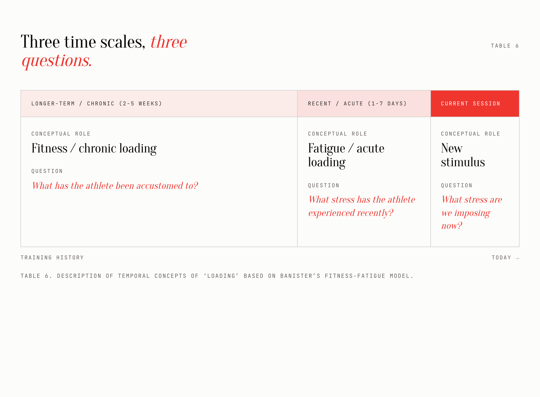
These concepts should not be confused with a claim that any single rolling load calculation precisely measures fitness or fatigue. They are simply temporal concepts within a theoretical model. The practical monitoring question remains whether the current stimulus and recent history are meaningfully different for this athlete and how the athlete responds (Impellizzeri et al., 2019; Impellizzeri et al., 2022).

Putting Changes in Training Load into the Context of Typical Variability

Consider an arbitrary summative whole body workload measure expressed in arbitrary units (AU). In this example, the identified change in workload is being determined by comparing the percent change to between-session CV percentage.  

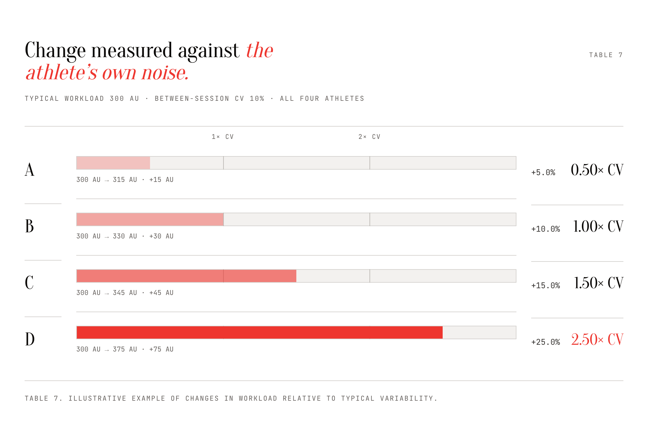
This illustrates why absolute change and percentage change are useful, but incomplete. A 15% increase tells us how much workload changed relative to the reference value. The CV tells us how the metric typically varies within a given individual (and their integrated microtechnology unit). Putting the two together gives us a way to consider signal relative to noise.

The 1×CV and 2×CV framing should be treated as a practical heuristic rather than a universal statistical threshold. The broader principle is that an observed change becomes more compelling as it moves farther beyond the athlete’s typical variability (Harry et al., 2024; Robertson et al., 2017).

When Is a Change Actually Meaningful?

A statistical flag is not a decision, but it is an invitation to investigate.

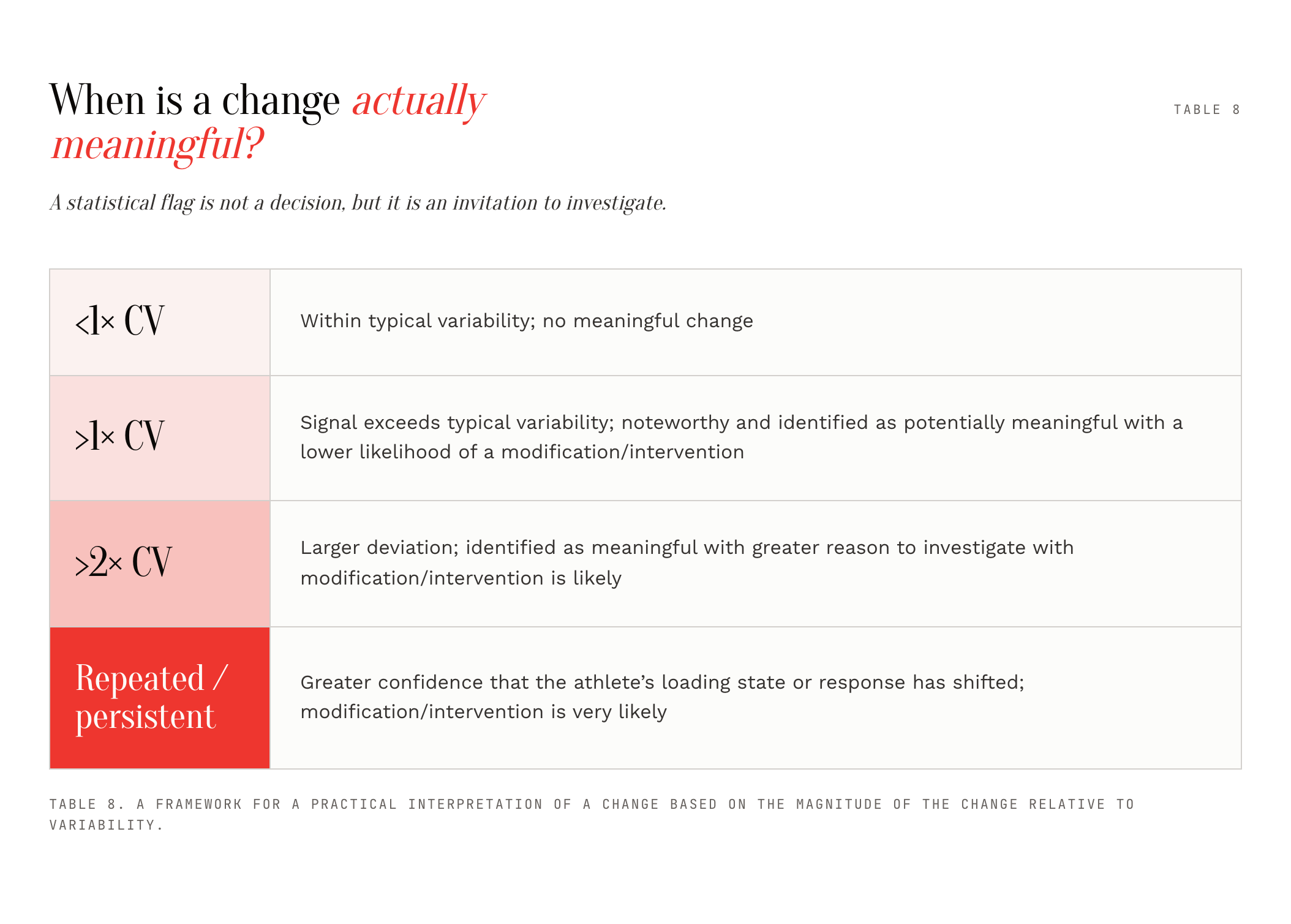
The farther an observed change moves beyond an athlete’s typical variability, the more attention it deserves. But the appropriate response depends on the question, the quality of the measurement, the magnitude and direction of the change, and the surrounding context.

Identifying Changes in Training Load Variables – Within Individual Z-Scores

For training stress, I separate the descriptive use of the CV from the operational use of the within-individual z-score. The CV can describe time-matched between session variability, while the z-score directly quantifies how unusual the current workload is relative to the athlete’s rolling, context-matched distribution.

Z-Score = (current individual daily value − individual rolling daily average) / individual rolling daily standard deviation

The comparison should be matched to the relevant time point. For example, GD-4 compared with previous GD-4 observations. The same principle can be applied to weekly values using game week-matched rolling reference points.

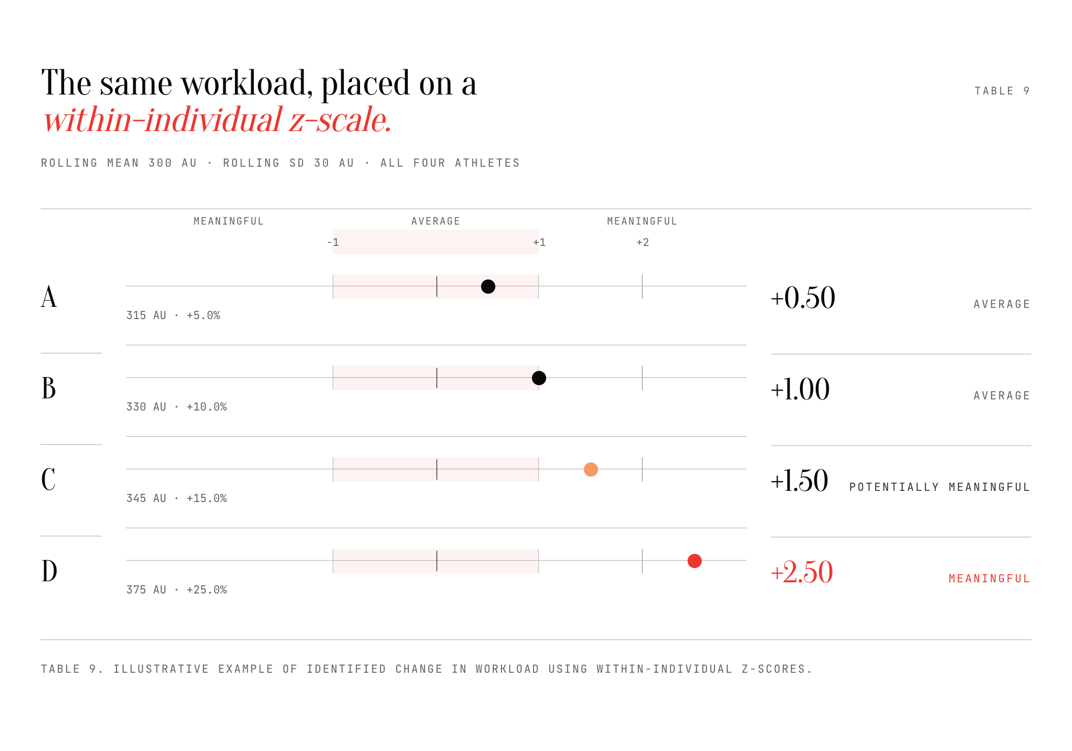
In this framework, values within ±1 z-score are considered average, values between ±1 and ±2 are potentially meaningful, and values beyond ±2 are meaningful. These categories are intended to support interpretation and investigation, not to replace practitioner judgment.

The rolling timeframe is context dependent and should align with the phase of training and similar time points. For example, if GD-4 occurs during a short week, it may be inappropriate to use that observation as part of the reference distribution for subsequent standard weeks.

The Same Workload Can Look Different Depending on the Reference Point

Consider an athlete whose current GD-4 workload is 350 AU. The conclusion changes depending on whether the comparison is made against all training days or against previous GD-4 sessions.

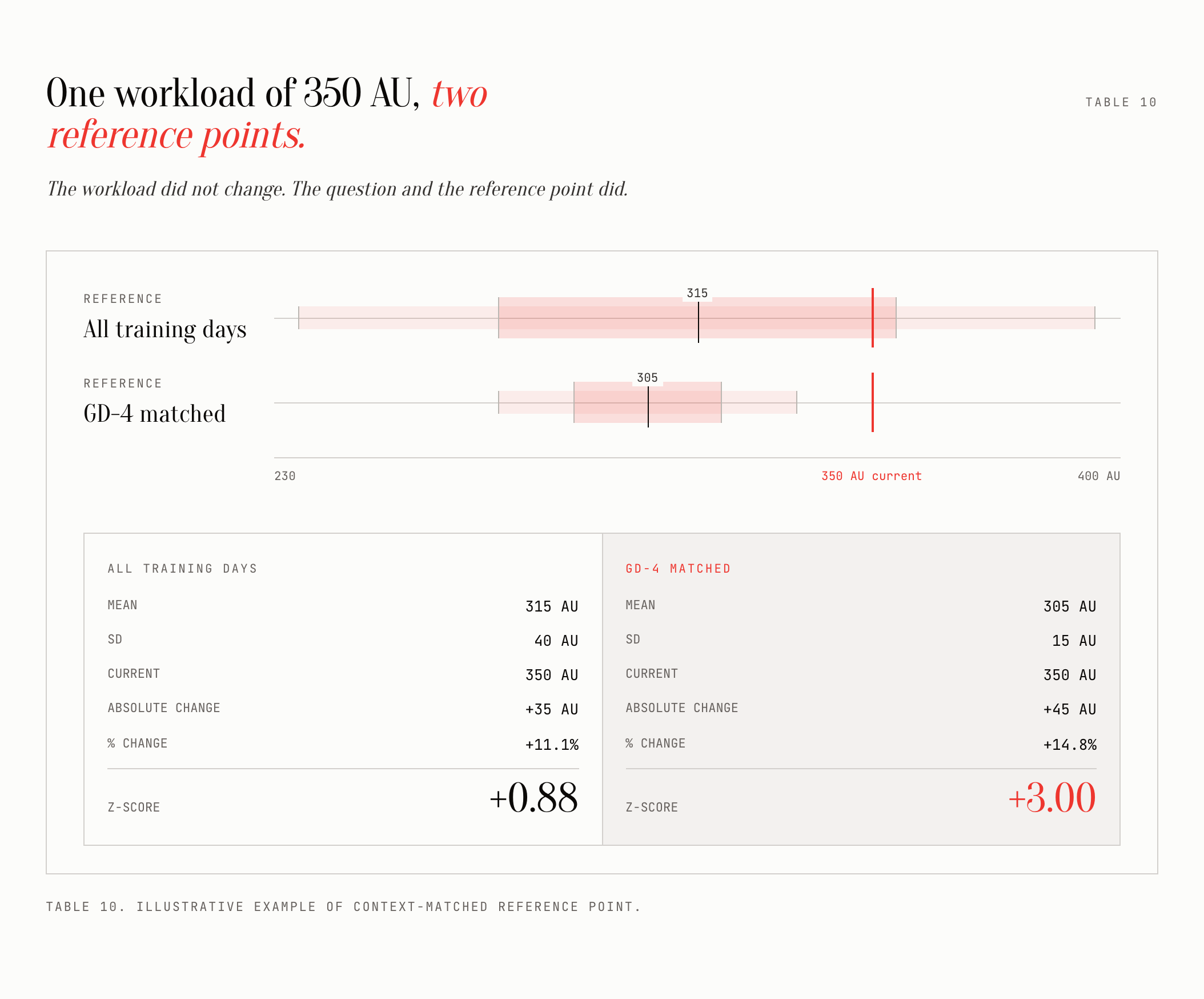
When using all the training days as the reference point, the workload looks relatively ordinary. However, when using the GD-4 reference point, it is three standard deviations above the athlete’s rolling GD-4 average. In other words, it is significantly higher of a workload on that particular day relative to the athlete’s norm.

In this example, the workload did not change, but the question and reference point changed. This is why time and context matching matters. The appropriate reference point is not necessarily the one with the largest sample size, rather it’s the one that best represents the comparison you are trying to make and is going to best support decision-making within your environment. 

Identifying Change in Subjective Response Indicators

The same logic applies to subjective response data (to better understand these terms check out this article). In my applied work, I use the wellness questionnaire adapted from McLean et al. (2010). It assesses general stress, fatigue, mood, sleep quality, and general muscle soreness. Each factor is scored from 1–5, producing an overall score out of 25 with higher scores representing better perceived wellness.

The questionnaire is useful because it captures several subjective dimensions of the athlete’s response rather than reducing wellness to a single question. Moreover, it is short and time efficient which makes it operationally feasible within a team sport environment. In my monitoring system, these data are analyzed using within-individual daily z-scores with rolling values defined in relation to relevant phases and time points.

McLean et al. (2010) used individual player z-scores for perceptual measures to account for different individual response patterns and reported historical reference data across players. Their work also demonstrated that perceptual measures changed across different between-match microcycles, reinforcing the importance of interpreting wellness in relation to the training and competition context.

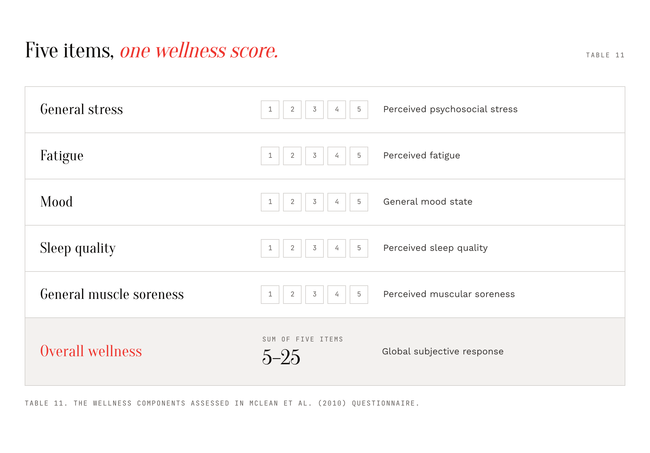
A score of 19/25 is therefore not inherently “good” or “bad” in isolation. The more useful question is whether 19 is unusual for this athlete, under these circumstances, and whether the change converges with other information.

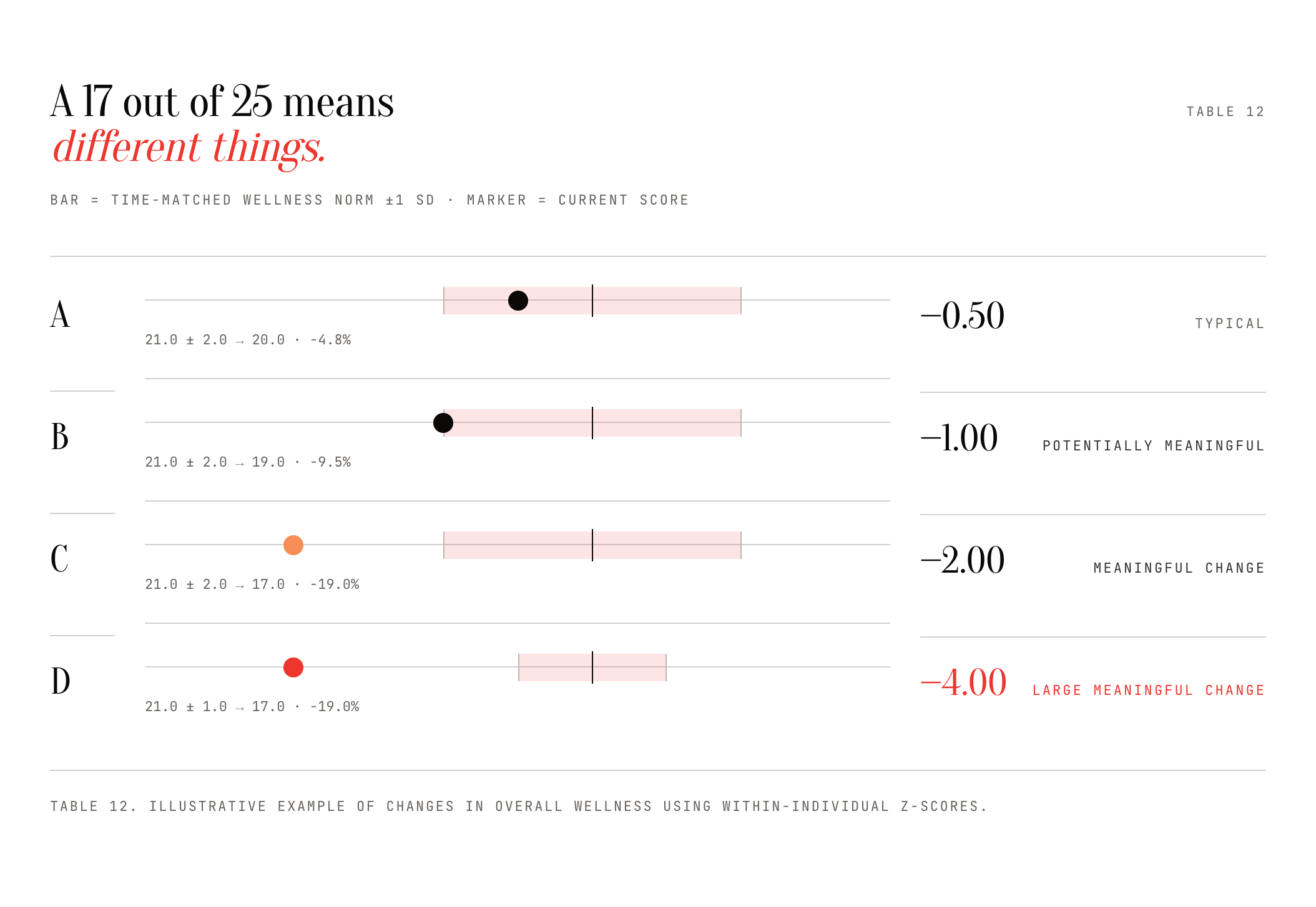
The point in this example is that the same raw score or percentage change can represent very different information depending on the athlete’s own reference point. This illustrates an example of the context-matched reference point being applied to wellness data. If a particular day in the microcycle has a predictable response pattern, comparing that day with previous comparable observations can provide a more relevant reference point than comparing it with every wellness observation the athlete has ever recorded.

Putting it all Together

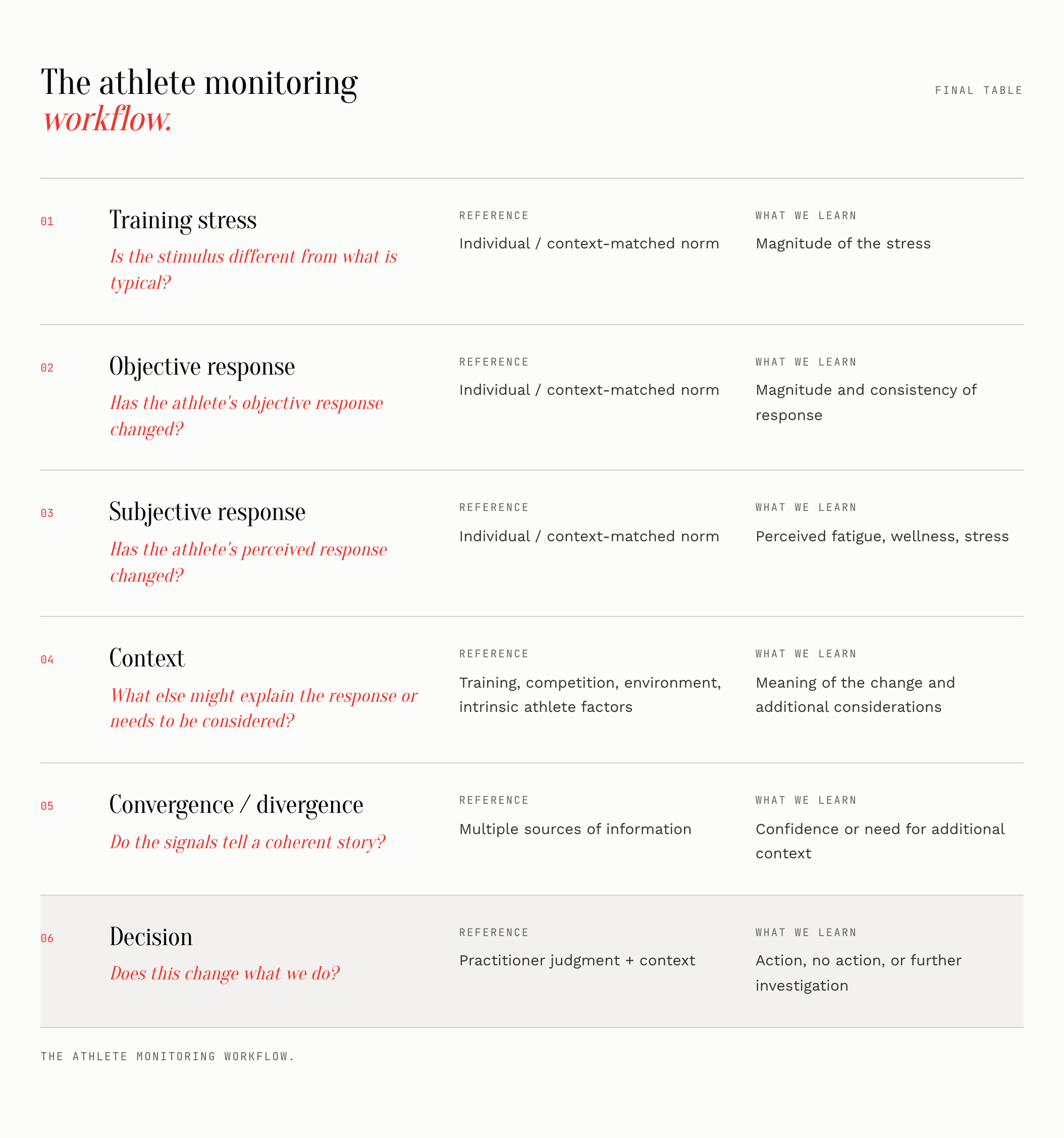
Identifying an athlete experiencing an increase in training load is useful, but it is just the starting point to painting a picture of the stress-response relationship within an athlete and ultimately supporting the decision-making process (Rebelo et al., 2026; Robertson et al., 2017).

The stress-response relationship asks whether the athlete’s observed response changed following the increase in training load. That response can be objective, subjective, or both. The same loading stimulus can produce different responses in different athletes, as well as different responses in the same athlete at different times.

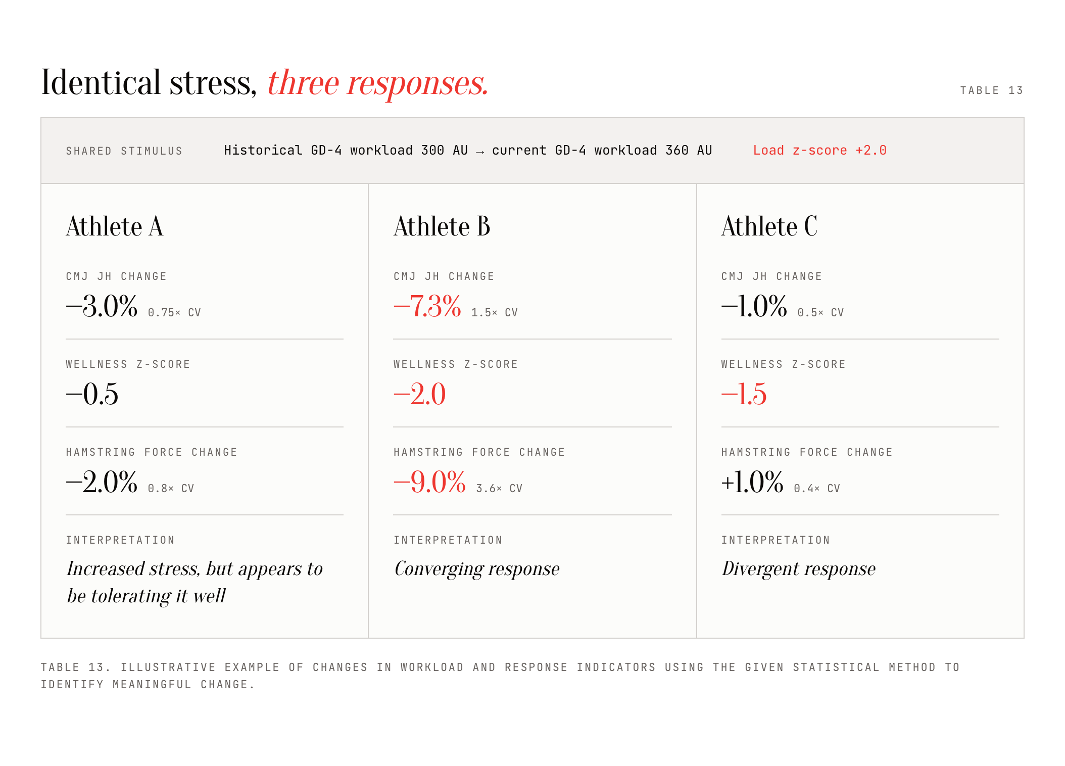
The method used to characterize meaningful change should reflect the nature of the measure and the reference data available. For training load and subjective wellness, within-individual z-scores can characterize how unusual a current observation is relative to the athlete's historical distribution. For measures such as CMJ and hamstring force, percentage change becomes more informative when interpreted relative to the measure's typical variability. In other words, the magnitude of change alone is insufficient; we need to understand that change in relation to what is typical for that athlete.

While the loading change is identical in this example, the athlete response to that loading change is not. Athlete B provides converging evidence with an increased in workload and multiple response indicators moving in the same direction illustrating a greater amount of fatigue is present than normal for his GD-4. Athlete C provides a more divergent picture with an increased workload, but objective response indicators remaining relatively stable while subjective wellness declined. Convergence increases confidence in the interpretation, while divergence increases the need for context and additional information.

While neither pattern automatically dictates an intervention, the monitoring system has generated a more useful question regarding how the observed stress and response should be interpreted in the context of this specific athlete?

Convergence versus Divergence

When multiple objective and subjective response indicators move in a consistent direction, confidence in the interpretation increases. When indicators disagree, it allows for additional questions to be asked and for more context to be used to gain insight into the observations.

For example, increased workload combined with reductions in CMJ performance, hamstring force, wellness, and sleep quantity provides a more coherent interpretation than an isolated reduction in one variable. Conversely, an unusual workload accompanied by stable objective and subjective response measures may suggest that the athlete tolerated the stimulus without an obvious change in the measured response. Therefore, divergence should allow for more questions to be asked rather than an automatic intervention or disregarding the data. It should prompt questions about additional context, measurement quality, the athlete’s recent training history, environmental factors, recovery behaviors, life and social factors, and potentially a host of other questions.

References

Bernards, J. R., Sato, K., Haff, G. G., and Bazyler, C. D. (2017). Current research and statistical practices in sport science and a need for change. Sports, 5(4), 87.

Harry, J. R., Hurwitz, J., Agnew, C., and Bishop, C. (2024). Statistical tests for sports science practitioners: Identifying performance gains in individual athletes. Journal of Strength and Conditioning Research, 38(5), e264–e272.

Hopkins, W. G. (2004). How to interpret changes in an athletic performance test. Sportscience, 8, 1–7.

Impellizzeri, F. M., Marcora, S. M., and Coutts, A. J. (2019). Internal and external training load: 15 years on. International Journal of Sports Physiology and Performance, 14(2), 270–273.

Impellizzeri, F. M., Jeffries, A. C., Weisman, A., Coutts, A. J., McCall, A., McLaren, S. J., and Kalkhoven, J. (2022). The ‘training load’ construct: Why it is appropriate and scientific. Journal of Science and Medicine in Sport, 25(5), 445–448.

McLean, B. D., Coutts, A. J., Kelly, V., McGuigan, M. R., and Cormack, S. J. (2010). Neuromuscular, endocrine, and perceptual fatigue responses during different length between-match microcycles in professional rugby league players. International Journal of Sports Physiology and Performance, 5, 367–383.

Rebelo, A., Bishop, C., Thorpe, R. T., Turner, A. N., and Gabbett, T. J. (2026). Monitoring training effects in athletes: A multidimensional framework for decision-making. Sports Medicine, 56(7), 1603–1624.

Robertson, S., Bartlett, J. D., and Gastin, P. B. (2017). Red, amber, or green? Athlete monitoring in team sport: The need for decision-support systems. International Journal of Sports Physiology and Performance, 12(Suppl 2), S273–S279.

Ward, P., Coutts, A. J., Pruna, R., and McCall, A. (2018). Putting the “I” back in team. International Journal of Sports Physiology and Performance, 13(8), 1107–1111.